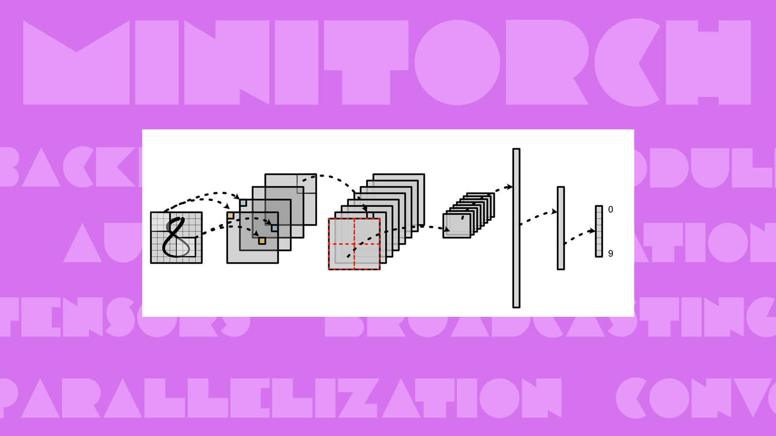
miniTorch

"Hmm, I wonder how PyTorch works?"

[GitHub Repo]

---

miniTorch is a Python re-implementation of the Torch API designed to be simple, easy-to-read, tested, and incremental. The final library can run Torch code. It is designed for me and anyone like me who wants to learn how deep learning libraries work under the hood. It is not intended to be super fast and well-optimized, but the implementation is still considerably efficient.

Feature Highlights

• Build models in an OOP way, just like PyTorch
• Variable wrapper around NumPy tensor
• Automatic differentiation
• JIT compilation
• GPU acceleration

Overview

Before diving into the implementation details, let's take a quick recap of the basic concepts in deep learning. In deep learning, we usually have a model defined as a certain network structure plus the parameters associated with the network. The model is trained by feeding some input data, performing some computation on the input data according to the defined network structure and the parameters, producing some output data, comparing the output data with the ground truth, and updating the model parameters to minimize the loss between the output data and the ground truth. This process is called backpropagation, which is essentially the chain rule in calculus.

Overview of Training a Deep Learning Model

So, given the above overview, we can see that the core of a deep learning library is to provide a way to define a model, perform computation on the model, and compute the gradients of the model parameters. To follow the implementation of PyTorch, miniTorch has the following TODOs:

• We need a data structure to represent the model: miniTorch implements a tree data structure Module that can be walked to find all of the parameters.
• We need to extend the functionality of a numerical value in Python: miniTorch implements a Variable class that wraps a NumPy data structure and provides additional functionalities for automatic differentiation such as storing the function that produces the value.
• We need to implement the computation graph: By connecting the variables through the functions between them, we can build a computation graph. miniTorch implements backpropagation by traversing the computation graph in reverse topological order.
• We need to improve the efficiency: First, miniTorch implements a Tensor class that avoids unnecessary for loops. Second, miniTorch needs parallel computation for it to be fast on CPU as well as GPU.

0. Module and Parameter

A deep learning model is often huge in size and complex in structure. For example, there are 1.7 trillion parameters in GPT-4. Also, it is common that a large and complex model contains several repeated structures such as Transformer blocks in GPT-4. A data structure is, therefore, needed for handling deep learning models that can abstract the model structure and parameters.

In software development, modular programming has been a common practice for a long time. It is a software design technique that emphasizes separating the functionality of a program into independent, interchangeable modules. In deep learning, we can also apply this technique to the model design. We can define a module as a self-contained piece of a model that can be connected to other modules to form a larger model.

Module is a recursive tree data structure. Inside each Module, we have the parameters and other sub-modules. This design is very similar to the tree data structure. We can define a Module class that has a list of sub-modules and a list of parameters. We can also define a Parameter class that has a value and a gradient. The Module class can be walked to find all of the parameters.

Let's take a look at an example of using Module and Parameter to define a model.

class MyModule(minitorch.Module):
    def __init__(self):
        super().__init__()
        self.parameter1 = minitorch.Parameter(15)
        self.apple1 = Apple()
        self.banana2 = Banana()

class Apple(minitorch.Module):
    def __init__(self):
        super().__init__()
        self.banana1 = Banana()
        self.banana2 = Banana()
        self.sweet = minitorch.Parameter(400)

class Banana(minitorch.Module):
    def __init__(self):
        super().__init__()
        self.yellow = minitorch.Parameter(-92)

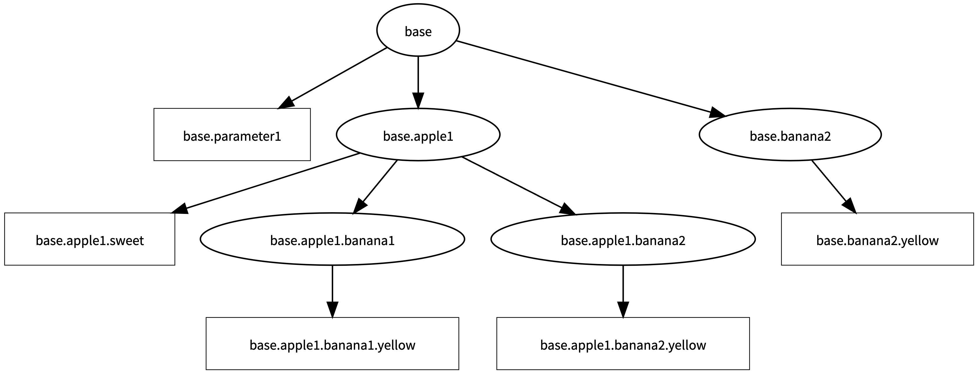
We can print the parameters of module MyModule like we are printing a tree.

{
  "parameter1": "15",
  "apple1.sweet": "400",
  "apple1.banana1.yellow": "-92",
  "apple1.banana2.yellow": "-92",
  "banana2.yellow": "-92"
}

Below is the tree structure of the module.

1. Automatic Differentiation through a Variable Wrapper

To update the parameters (a.k.a. learn the model), we need to compute the gradients of the parameters given the computed loss and update them for gradient descent. The gradients can be computed by backpropagation, which is essentially the chain rule in calculus. The chain rule is a method for finding the derivative of composite functions. For example, given a composite function f(g(x)), the derivative of f(g(x)) is f'(g(x)) * g'(x). The chain rule can be applied to the computation graph of a deep learning model. The computation graph is a directed acyclic graph (DAG) where the nodes are the variables and the edges are the functions that produce the variables.

But there is one gigantic problem remaining: how to compute the derivative of a function? There are several options:

• symbolic differentiation: By deriving the derivative of a function symbolically, we can compute the derivative of the function. However, it is not always easy to derive the derivative of a function symbolically.
• numerical differentiation: Since the derivative of a function is the slope of the tangent line of the function, we can approximate the derivative of a function by computing the difference between two points on the function. However, it might be costly since we need to compute the function twice. Below is the code snippet of numerical differentiation.

def central_difference(f: Any, *vals: Any, arg: int = 0, epsilon: float = 1e-6) -> Any:
    """
    Args:
        f : arbitrary function from n-scalar args to one value
        *vals : n-float values $x_0 \ldots x_{n-1}$
        arg : the number $i$ of the arg to compute the derivative
        epsilon : a small constant

    Returns:
        An approximation of $f'_i(x_0, \ldots, x_{n-1})$
    """
    # f(x + epsilon)
    x_vals_1: List[Any] = list(vals)
    x_vals_1[arg] = x_vals_1[arg] + epsilon
    # f(x - epsilon)
    x_vals_2: List[Any] = list(vals)
    x_vals_2[arg] = x_vals_2[arg] - epsilon

    return (f(*x_vals_1) - f(*x_vals_2)) / (2 * epsilon)

In miniTorch and other DL libraries, we adopt another solution, namely automatic differentiation. The idea is to decompose a function and gather the steps about the computational paths within a function. Then, we can compute the derivative of each elementary function and apply the chain rule to compute the derivative of the composite function.

For example, if we are going to calculate the derivative of the function, (x * x) * y + 10.0 * x + y, w.r.t. both x and y, we can decompose the function into several elementary functions and construct the computation path as follows (ignore the random numbers inside the circles):

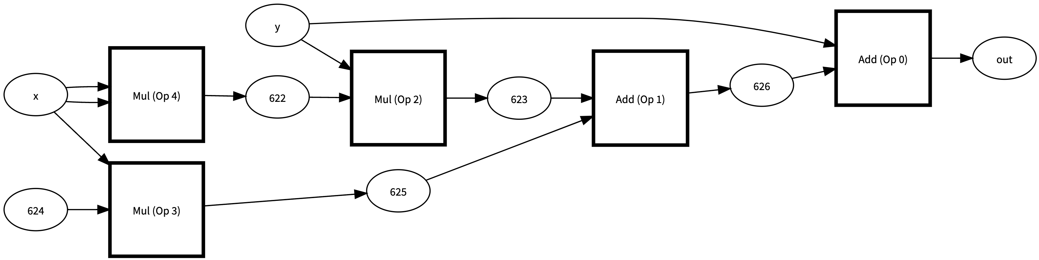
However, in order to build such a computation path, we need to trace all the internal computation of any function - which can be difficult to do because Python does not directly expose how its inputs are used in the function, i.e. given the input of a function, what we get is only the output, but not the calculation process of the input inside the function.

The solution is quite beautiful:

• Build a new data structure Variable to replace the original numerical value in Python.
• Overload the operators in Python with Functions to make the Variable class behave like a numerical value.
• Extend the functionality of the Variable class to store the function that produces the value.

One of the benefits of such a design is that for the user, the Variable class behaves like a numerical value, so the user can use it just like a numerical value and never need to know what is happening under the hood.

Implementation of autodiff

To achieve what I just described above, we need to implement the code architecture shown in the flowchart below. The code can be found in these three files: scalar.py, scalar_function.py, and autodiff.py.

Implementation of Automatic Differentiation on Scalar

The ScalarFunction class can be viewed as the Functions class as we described above.

• It overloads the operators in Python and provides additional functionalities for automatic differentiation such as creating new Scalar objects and storing the function that produces the value.
• Inside each inherited class of ScalarFunction, (e.g., Add, Mul, etc.), we need to implement the forward and backward methods. The forward method computes the value of the function given the input Scalar objects. The backward method computes the derivative of the function w.r.t. the input Scalar objects.
• After computing the result(s) of the function, apply method also creates a new Scalar object and stores the function and the input scalars that produces the value in the Scalar object. This is the key to automatic differentiation. By storing the function that produces the value, we can trace the computation path and compute the derivative of the composite function by applying the chain rule.
• When computing the derivatives, sometimes we need to access the value from the forward pass. We can use the ctx object to store the value from the forward pass and access it in the backward pass.
• For example, The derivative of sigmoid(x) with respect to x is sigmoid(x) * (1 - sigmoid(x)). Therefore, the Sigmoid class can be implemented as follows:

class Sigmoid(ScalarFunction):
@staticmethod
def forward(ctx: Context, a: float) -> float:
    sig = operators.sigmoid(a)
    ctx.save_for_backward(sig)
    return sig

@staticmethod
def backward(ctx: Context, d_output: float) -> float:
    (sig,) = ctx.saved_values
    result: float = sig * (1 - sig) * d_output
    return result

The core Scalar class can be viewed as the Variable class as we described above. It wraps a Python float object and provides additional functionalities for automatic differentiation with overloaded operators.

• A Scalar object contains a data attribute that stores the value of the Scalar object.
• It also stores the history that contains the ScalarFunction that produces the current Scalar object.
• By calling the chain_rule method, we can compute the derivative w.r.t. the input Scalar object that produces this Scalar object.

Backpropagation

Now, we have a computation graph constructed by Scalar objects and ScalarFunction objects, and we can compute the derivative at each node in the computation graph by applying the chain rule. Next, we need to figure out how to backpropagate the derivative from the output node to the input node. That is, we need to find a way to traverse the computation graph in reverse order to accumulate the gradients so that we can update the parameters of the DL model (which would be the leaves of the computation graph).

We could just apply these rules randomly and process each nodes as they come aggregating the resulted values. However this can be quite inefficient. It is better to wait to call backward until we have accumulated all the values we will need.

To handle this issue, we will process the nodes in topological order. The topological ordering of a directed acyclic graph is an ordering that ensures no node is processed after its ancestor. Once we have the order defined, we process each node one at a time in order.

Algorithm:

def topological_sort(variable: Variable) -> Iterable[Variable]:
    """
    Computes the topological order of the computation graph.

    Args:
        variable: The right-most variable

    Returns:
        Non-constant Variables in topological order starting from the right.
    """
    visited: List[int] = list()
    ordered_vars: List[Variable] = list()

    def visit(variable: Variable) -> None:
        if variable.is_constant() or variable.unique_id in visited:
            return
        if not variable.is_leaf():
            for input_var in variable.parents:
                visit(input_var)
        visited.append(variable.unique_id)
        ordered_vars.insert(0, variable)

    visit(variable)
    return ordered_vars


def backpropagate(variable: Variable, deriv: Any) -> None:
    """
    Runs backpropagation on the computation graph in order to
    compute derivatives for the leave nodes.

    Args:
        variable: The right-most variable
        deriv  : Its derivative that we want to propagate backward to the leaves.

    No return. Should write to its results to the derivative values of 
    each leaf through `accumulate_derivative`.
    """
    ordered_vars: Iterable[Variable] = topological_sort(variable)
    # Record the derivative of each variable
    derivatives: Dict[int, Any] = {var.unique_id: 0 for var in ordered_vars}
    derivatives[variable.unique_id] = deriv

    for var in ordered_vars:
        if var.is_leaf():
            var.accumulate_derivative(derivatives[var.unique_id])
        else:
            for parent_var, deriv in var.chain_rule(derivatives[var.unique_id]):
                if parent_var.is_constant():
                    continue
                if parent_var.unique_id in derivatives:
                    derivatives[parent_var.unique_id] += deriv
                else:
                    derivatives[parent_var.unique_id] = deriv

2. A More Efficient Variable Wrapper: Tensor

We now have a fully developed autodifferentiation system built around scalars. This system is correct, but it is inefficient during training, since every scalar number requires building an object, and each operation requires storing a graph of all the values that we have previously created. Moreover, training requires repeating the above operations, and running models, such as a linear model, requires a for loop over each of the terms in the network.

In miniTorch, a new variable wrapper class Tensor is implemented to solve these problems. Tensors group together many repeated operations to save Python overhead and to pass off grouped operations to faster implementations.

What's under the hood of Tensor?

Under the hood, a Tensor is a multi-dimensional array of numbers. It is a wrapper around a NumPy array. Most importantly, it separates the actual data storage from the tensor object. This allows us to share the data storage between multiple tensors. For example, we can create a tensor a and a tensor b that is a view of a. They share the same data storage. Then, we can perform some operations on a and b without creating new tensors. This is very useful when we are dealing with large tensors.

As shown in the chart below, the Tensor class extends what we have built for Scalar.

Implementation of Tensor

Notice what is different (marked in purple):

• We have a TensorData class whose _storage stores the actual data of the tensor. The different tensors can share the same data storage, but come with different _stride and _shape.
• We have a TensorBackend class which collects all the functions that can be applied to the tensor. The TensorBackend class is a strategy pattern. It allows us to switch between different implementations of the tensor functions by changing the ops objects. For example, we can implement the higher-ordered functions in a for loop manner (see tensor_ops.py), or with numba JIT parallel computation (see fast_ops.py), or with CUDA GPU computation (see cuda_ops.py).

Let's take a look at an example of calling Permute on a tensor and how it works in autodiff with the new Tensor class. Inside the Permute Function, the forward will create a new Tensor with the same data storage but different _stride and _shape. (i.e. different TensorData but with the same _storage). The backward will do something similar.

tensor_functions.py:

...

class Permute(Function):
    @staticmethod
    def forward(ctx: Context, a: Tensor, order: Tensor) -> Tensor:
        ori_order: List[int] = [int(i) for i in order._tensor._storage]
        ctx.save_for_backward(a, ori_order)
        return minitorch.Tensor(a._tensor.permute(*ori_order), backend=a.backend)

    @staticmethod
    def backward(ctx: Context, grad_output: Tensor) -> Tuple[Tensor, float]:
        (a, ori_order) = ctx.saved_tensors
        order: List[int] = [ori_order.index(i) for i in range(len(ori_order))]
        grad_output = minitorch.Tensor(
            grad_output._tensor.permute(*order), backend=a.backend
        )
        return grad_output, 0
...

tensor.py:

from .tensor_functions import Permute
...
class Tensor:
    ...
    def permute(self, *order: int) -> Tensor:
        "Permute tensor dimensions to *order"
        return Permute.apply(self, tensor(list(order)))
    ...

tensor_data.py:

class TensorData:
    ...
    def permute(self, *order: int) -> TensorData:
        """
        Permute the dimensions of the tensor.

        Args:
            order (list): a permutation of the dimensions

        Returns:
            New `TensorData` with the same storage and a new dimension order.
        """
        assert list(sorted(order)) == list(
            range(len(self.shape))
        ), f"Must give a position to each dimension. Shape: {self.shape} Order: {order}"

        # TODO: Implement for Task 2.1.
        return TensorData(
            storage=self._storage,
            shape=tuple(self.shape[i] for i in order),
            strides=tuple(self._strides[i] for i in order),
        )
...

What is a little bit tricky is that unlike Scalar, we might want to deal with operations that work on tensors with different shapes. For example, we might want to add a float value 1.0 to a tensor of shape (3, 2). In this case, we need to broadcast the tensors to the same shape. We have the following rules for broadcasting:

• Rule 1: Dimension of size 1 can be broadcasted to any shape.
• Rule 2: Extra dimensions of 1 can be added with view.
• Rule 2: Zip automatically adds dims of size 1 on the left.

Therefore, we can implement the shape_broadcast method as follows:

def shape_broadcast(shape1: UserShape, shape2: UserShape) -> UserShape:
    """
    Broadcast two shapes to create a new union shape.

    Args:
        shape1 : first shape
        shape2 : second shape

    Returns:
        broadcasted shape

    Raises:
        IndexingError : if cannot broadcast
    """
    # Rule 3: extra dimensions of 1 can be implicitly added to the left of the shape.
    if len(shape1) > len(shape2):
        shape2 = [1 for _ in range(len(shape1) - len(shape2))] + list(shape2)
    else:
        shape1 = [1 for _ in range(len(shape2) - len(shape1))] + list(shape1)
    # Now, shape1 and shape2 have the same dimension.
    n_shape: List[int] = []
    for i in range(len(shape1)):
        if shape1[i] != shape2[i]:
            # Rule 1: dimension of size 1 broadcasts with anything
            if shape1[i] == 1:
                n_shape.append(shape2[i])
            elif shape2[i] == 1:
                n_shape.append(shape1[i])
            else:
                raise IndexingError(f"Cannot broadcast {shape1} and {shape2}.")
        else:
            n_shape.append(shape1[i])
    return tuple(n_shape)

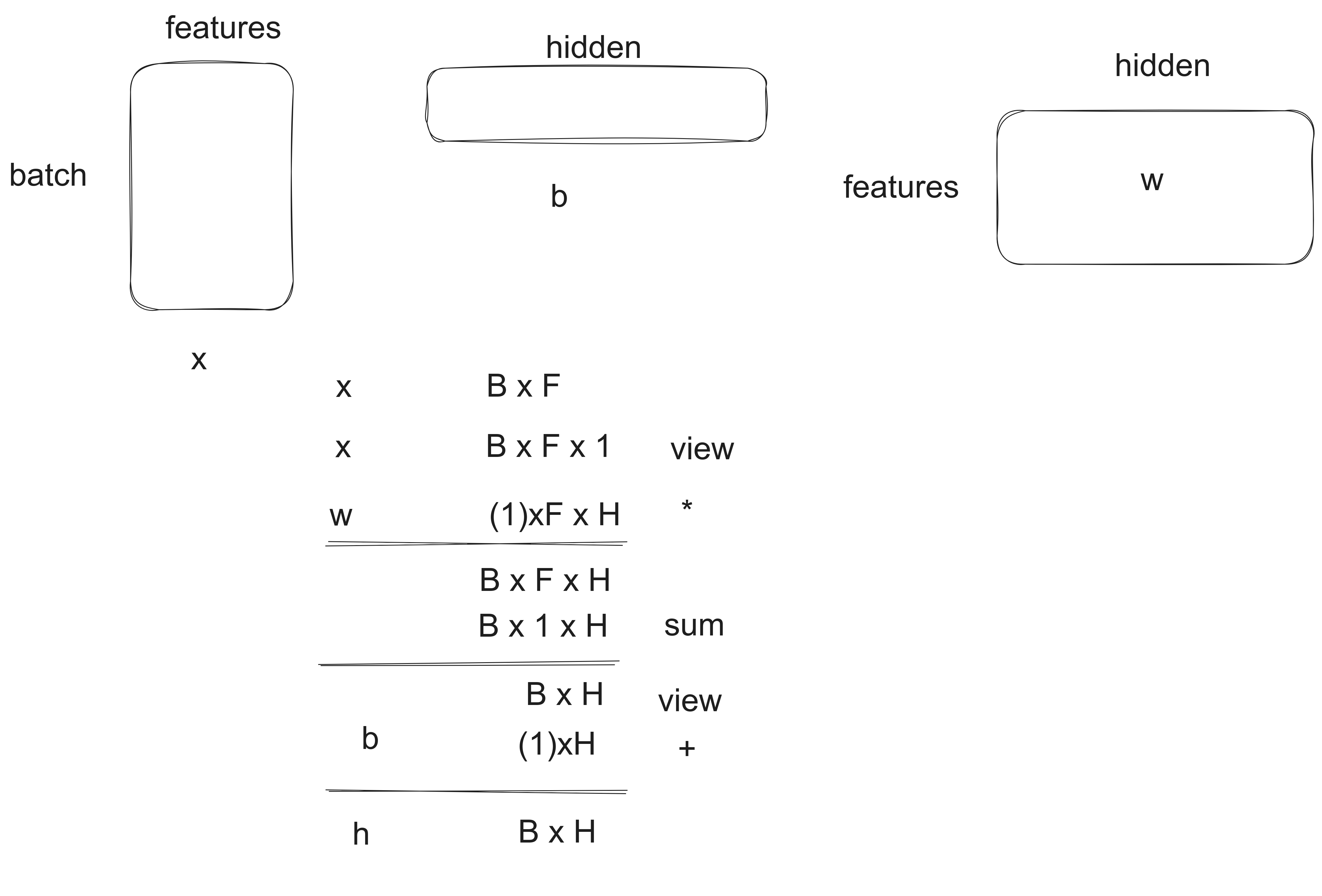
For example, in the case of linear model, we have the data X of shape (B * F), the weight W of shape (F * H), and the bias b of shape (H). To compute the output Y following Y = X @ W + b, we need to follow the following steps (suppose we don't have matrix multiplication implemented):

3. Parallel Computation on CPU and GPU

[To Be Updated]